
Dr Phill
Dr Phill
Machine leaning has a number of application and implementations. One of the most well known is the Neural Network.
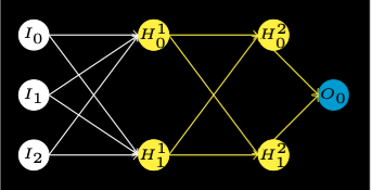
A neural network emulates the function of a brain. It has interconnected artificial neurons in three or more layers.
Information from the outside world enters the artificial neural network from the input layer. Input nodes process the data, analyze or categorize it, and pass it on to the next layer.
Hidden layers take their input from the input layer or other hidden layers. Artificial neural networks can have a large number of hidden layers. Each hidden layer analyzes the output from the previous layer, processes it further, and passes it on to the next layer.
Each hidden layer must have the same number or fewer neurons than the number of inputs. For three inputs, two neurons is a good choice. Each neuron must have a weight \(w_i\) for each input \(x_i\). It must also have a bias \(b\). Each weight and the bias are initially assigned a random number \([0, 1)\).
Neurons have a non-linear, differentiable, activation function \(\phi\) that maps the weighted inputs to an number \([0, 1]\). A good choice of activation function also has a convenient derivative.
\[\phi(x) = \frac{1}{1 + e^{-x}}\quad \frac{d\phi(x)}{dx} = \phi'(x) = -\frac{e^{-x}}{(1 + e^{-x})^2} = \phi(x)(1 - \phi(x)) \]
\[\frac{d\phi(\alpha(x))}{dx} = \alpha'(x)\phi'(\alpha(x))\]
The output layers give the final results of all the data processing by the artificial neural network. It can have single or multiple nodes. For instance, if we have a binary (yes/no) classification problem, the output layer will have one output node, which will give the result as 1 or 0. It can have multiple values. However, if we have a multi-class classification problem, the output layer might consist of more than one output node.
The Palmer Penguin dataset has data on three types of penguin. The data files can be found at Allison Horst Palmer Penguins as CSV files. There is data for 344 penguins on three species Adélie, Chinstrap, and Gentoo. The data has measurements of flipper length, beak (culmin) length, and beak (culmin) depth.
Observation of the data gives some differences between penguin species.
The MNIST data set is perhaps the most widely used example of neural networks. It consistes of images of hand written single digits 0-9. The idea is to train an neural network using the train data set and get a 98%+ score recognising the tk10 data. There are two data sets idx1 and idx3.
We are going to build a neural network to identify penguins by flipper length and culmin length and depth. We will use a subset of the penguin data for training and the full data set for testing.
We will start by building a simple neural network and then try and improve on it.
The penguin culmin and flipper measurements are in millimetres. These need to be converted to metres so that each measurement is less than one.
Each neuron needs to be able to calculate an activation function that is constrained as described.
The inputs for the first hidden layer are the inputs \(x_i\). For each neuron in the layer index \(k\) the weights \(w_{1ki}\) and the bias \(b_{1k}\) applied. The activation function is applied to give the inputs \(A_1k\) for the next layer.
\[\alpha_{1k} = \sum_i x_i w_{1ki} + b_{1k}\] \[A_{1k} = \phi(\alpha_{1k})\]
The inputs for the later hidden layers index \(j > 1\) are the activations from the previous layer \(A_{j-1,i}\). Where the index \(k\) from the previous layer has been replace by the index \(i\). For each neuron in the layer index \(k\) the weights \(w_{jki}\) and the bias \(b_{jk}\) applied. The activation is applied to give the inputs for the next layer.
\[\alpha_{jk} = \sum_i A_{j-1,i} w_{jki} + b_{jk}\] \[A_{jk} = \phi(\alpha_{jk})\]
The activation outputs from each neuron in a layer become the inputs for the next hidden layer or the output layer. This is called forward propagation.
The output layer is similar to a hidden layer.
The inputs for the output layers index \(n\) are the activations from the previous layer \(A_{ji}\). Where the index \(k\) from the previous layer has been replace by the index \(i\). For each neuron in the layer index \(k\) the weights \(w_{nki}\) and the bias \(b_{nk}\) applied. We calculate the predicted results \(\tau_k\) for each training penguin. The activation function is not applied.
\[\tau_k = \sum_i A_{ji} w_{nki} + b_{nk}\]
Now, we need to perform back propagation to modify the weights of the neurons. It is important to notice that the values of the activations of the hidden layers are no longer valid as they are calculated on a per training set basis.
We need to define a tunable learning rate that is often set to one \(l = 1\). The cost \(J_k\) is standard mean squared loss function from regression. This is summing over the output of each of the \(m\) training inputs. There is the expected true result \(T_k\) for each training penguin \(t = 1..m\).
\[J_k = \frac{1}{2m}\sum_t(\tau_k - T_k)^2\]
The reason why the diviser is \(2m\) rather than \(m\) is to cancel out the factor on \(2\) in the derivative. This is not an issue as the corrections are multiplied by a learning rate. This is tunable. It will be set to one \(l = 1\), but because of the factor of \(2\), it is effectively \(l = 0.5\).
Back propagation works by starting with the cost and work backwards through the network. For each neuron, we calculate the derivative of the cost function for each of the weights and the bias. Most of the derivatives require the neuron’s input activations and their derivatives. As there is a set of activations associates with each training penguin, we need to calculate the derivates for each set and then use the average to correct the weights and biases.
First take the derivative of the cost with respect to the predicted result \(\tau\). We will abbreviate the derivating to \(d\tau\).
\[d\tau_k = \frac{\partial J_k}{\partial\tau_k} = \frac{1}{m}\sum_t(\tau_k - T_k)\]
We now calculate the derivative of the cost with respect to each of the output layer weights \(w_{nki}\) using the chain rule.
\[\tau_k = \sum_i A_{ji} w_{nki} + b_{nk}\]
\[dw_{nki} = \frac{\partial J_k}{\partial w_{nki}} = \frac{\partial J_k}{\partial\tau_k} \frac{\partial\tau_k}{\partial w_{nki}} = d\tau_k A_{ji}\]
Now correct each weight.
\[w_{nki} = w_{nki} - \frac{l}{m}\sum_t d\tau_k A_{ji}\]
Use the same approach for the bias $b_{nk}.
\[db_{nk} = d\tau_k\]
\[b_{nk} = b_{nk} - l d\tau_k\]
The next stage is to back propagate though all but the first hidden layer. We need the derivitive of the cost with respect to the input activations from the next layer. Again, each \(A\) term needs to be the average of the derivatives for each training penguin. As \(A_{ji}\) is the input to all of the next layer neurons, it contributes to the cost of each of them and the costs need to be summed.
\[dA_{ji} = \sum_k w_{nki}d\tau_k\]
We also need the neuron activation equation. Remember that the \(i\) subscript of the next layer activation needs to revert to the \(k\) subscript, $dA_{ji} \(dA_{jk}\).
\[\alpha_{jk} = \sum_i A_{j-1,i} w_{jki} + b_{jk}\] \[A_{jk} = \phi(\alpha_{jk})\]
The derivatives with respect to the weights and bias are:
\[dw_{jki} = dA_{jk}A_{j-1,i}\phi'(\alpha_{jk})\]
\[db_{jk} = dA_{jk}\phi'(\alpha_{jk})\]
\[dA_{ji} = \sum_k dA_{jk} w_{jki} \phi'(\alpha_{jk})\]
The gradient of \(J\) for the first layer with respect to the weights \(u_i\) and bias \(b_1\) can be calculated.
\[dA_i = \frac{\partial J}{\partial A} = dB_i \frac{\partial B_i}{\partial A_i}\] \[dA_i = dB_i v_i\phi'(\beta_i)\] \[du_i = \frac{\partial J}{\partial u_i} = dA_i \frac{\partial A_i}{\partial u_i}\] \[\alpha_i = \Sigma x_i w_i + b\] \[A_i = \phi(\alpha_i)\] \[du_i = dA_i x_i \phi'(\alpha_i)\] \[db_1 = dA_i \phi'(\alpha_i)\]
The training process is iterative. We will tune the number of iterations.