Dr Phill’s Science Made Simple

Astro-Mathematics

Besselian Centre Line

The objective is to transform the besselian elements into the longitude and latitude coordinates of the eclipse centre line at any partcular time during the eclipse.

The Earth is an ellipsoid. The eccentricity \(e\) of the Earth meridian is required for calculations. The accepted value is \(e^2 = 0.00669454\).

Given the Besselian elements at Julian date \(t\) the latitude \(\phi\) and longitude \(\lambda\) of the intersection of the Moon shadow axis with the Earth’s surface are required.

The following diagrams shows the intersection of the fundamental plane and the shadow axis with the Earth’s surface. The eccentricity of the meridian is exagerated for clarity.

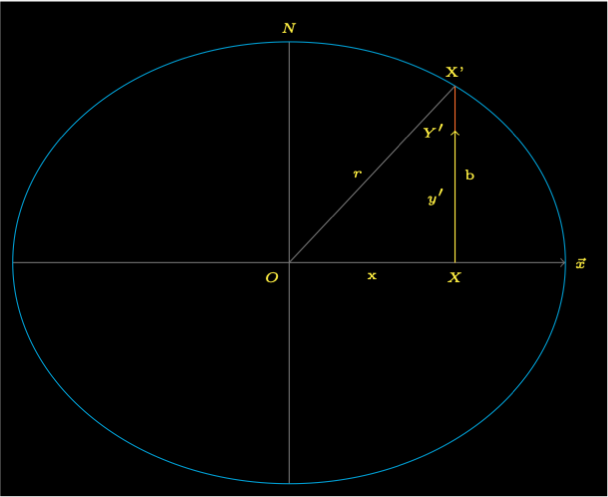
Figure 1: Earth Polar Plane Normal To Shadow Axis

Earth Polar Plane Normal To Shadow Axis

Figure 1: Earth Polar Plane Normal To Shadow Axis shows a slice through the Earth where \(O\) is the centre of the Earth and \(N\) is the North Pole. The horizontal axis is parallel to the fundamental plane’s X axis. The distance \(x\) is the Besselian element for time \(t\). The line \(XX'\) lies in the fundamental plane'. Where the point \(X'\) on the Polar place is a projection from the fundamental plane.

Calculate Ellipse Intersection and Latitude

Although the diagrams show the shadow axis, the calculations are generic. For umbral and penumbra points, the point on the line needs to be the shadow cone vertex.

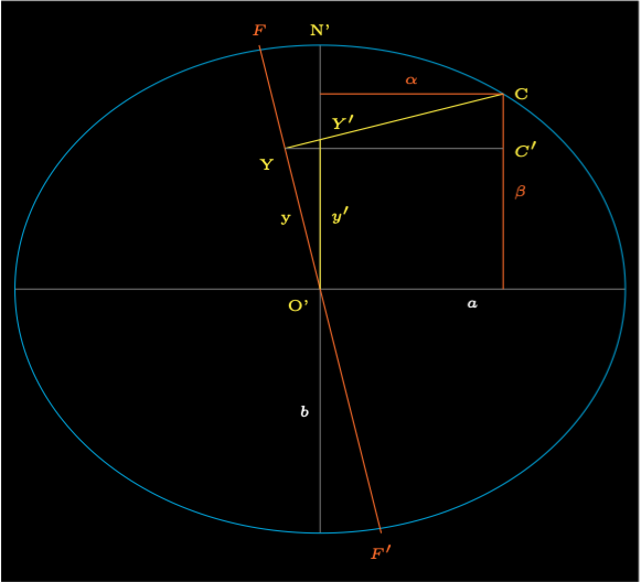
Figure 2: Fundamental Plane to Earth Surface Y-Z' Slice

Figure 2: Fundamental Plane to Earth Surface Y-Z' Slice shows the intersection plane. The intersection of the fundamental plane \(F'F\) with the Earth’s surface is an ellipse. It is in a plane perpendicular the the x axis and the line XX' lies in the plane. It has semi-major axis \(a\) and semi-minor axis \(b\). We will use the cartesian coordinates \((u, v)\) for this plane.

\(a^2 = 1 - x^2\)

\(b^2 = (1 - e^2)(1 - x^2)\)

The equation of the ellipse.

\[\frac{u^2}{(1 - x^2)} +\frac{v^2}{(1 - e^2)(1 - x^2)} = 1\]

Let \(\epsilon^2 = 1 - e^2\) and \(\xi^2 = 1 - x^2\). Reorganise Equation (1) at point \((\alpha, \beta)\).

\[\beta^2 = \epsilon^2\xi^2 - \alpha^2\epsilon^2\]

A line of gradient \(\gamma\) passing through point \((\rho, \sigma)\) at point \((\alpha, \beta)\).

\[\beta - \sigma = \gamma(\alpha - \rho)\]

Reorganise Equation (3) and square.

\[\beta^2= \gamma^2\alpha^2 + 2\gamma\alpha(\sigma - \gamma\rho) + (\sigma - \gamma\rho)^2\]

Subtract Equation (2) from Equation (4).

\[\alpha^2(\gamma^2 + \epsilon^2) + 2\alpha\gamma(\sigma - \gamma\rho) + (\sigma - \gamma\rho)^2 - \epsilon^2\xi^2 = 0\]

This is a quadratic equation in \(\alpha\). Set the variables to solve the quadratic equation.

\(a = \gamma^2 + \epsilon^2\)

\(b = 2\gamma(\sigma - \gamma\rho)\)

\(c = (\sigma - \gamma\rho)^2 - \epsilon^2\xi^2\)

\(d = b^2 - 4ac\)

If \(d < 0\) then the shadow axis misses the Earth and there is no eclipse.

Solve the quadratic equation for \(\alpha\) taking the positive square root as \(\alpha \ge 0\).

\[\alpha = \frac{-b + \sqrt{d}}{2a}\]

Calculate \(\beta\) from \(\alpha\) using Equation (3).

\[\beta = \gamma(\alpha - \rho) + \sigma\]

Figure 3: Plane through Earth centre, North pole, and shadow axis intersection

Plane through Earth centre

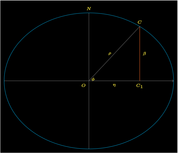
Figure 3: Plane through Earth centre, North pole, and shadow axis intersection shows the ellipse that is the plane through the points \(O\), \(N\), and \(C\). The radius of \(C\) is \(\rho\). The distance \(OC_1\) is \(\eta\).

The radius \(OC_1\) is:

\[\eta = \sqrt{(x^2 + \alpha^2)}\]

The latitude \(\phi\) is:

\[\phi = \tan^{-1}\left(\frac{\beta}{\eta}\right)\]

Figure 4: Earth Latitude Plane

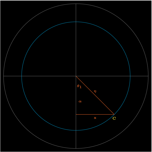
Figure 4: Earth Latitude Plane shows the plane of the latitude of where the shadow axis intersects the Earth’s surface. The radius of the circle of latitude is \(\eta\) and \(\theta_1\) is the longitude offset.

The point \(C = (\alpha, \beta)\) where the shadow axis intersects the Earth’s surface is at the intercection of the line \(YC\) and the ellipse.

\[\tan\theta_1 = \frac{x}{\alpha}\]

The longitude \(\lambda\) can be calculated from the value of \(\mu\). The Besselian \(\mu\) is in the range \(0 \le \mu < 2\pi\). It needs to be converted into the range \(-\pi < \mu \le \pi\). The longitude \(\lambda\) can be calculated.

\[\lambda = \theta_1 - \mu\]

Calculate the Shadow Axis Latitude and Longitude

The line \(CY\) is the shadow axis, where \(y\) and \(d\) are the Besselian elements at time \(t\). The Besselian element \(d = \widehat{CYC'} = \widehat{YO'Y'}\). The distance \(y' = y\sec d\) is the distance from the equator to the shadow axis. The shadow axis has gradient \(\gamma = \tan d\) and starts at point \(Y = ((\rho, \sigma)) = (0, y\sec d)\).

Use Equation (5) to Equation (11) to obtain the values of the latitude \(\phi\) longitude \(\lambda\).

The Umbral Cone

Figure 5: The Umbral Cone Width

The Umbral Cone Width

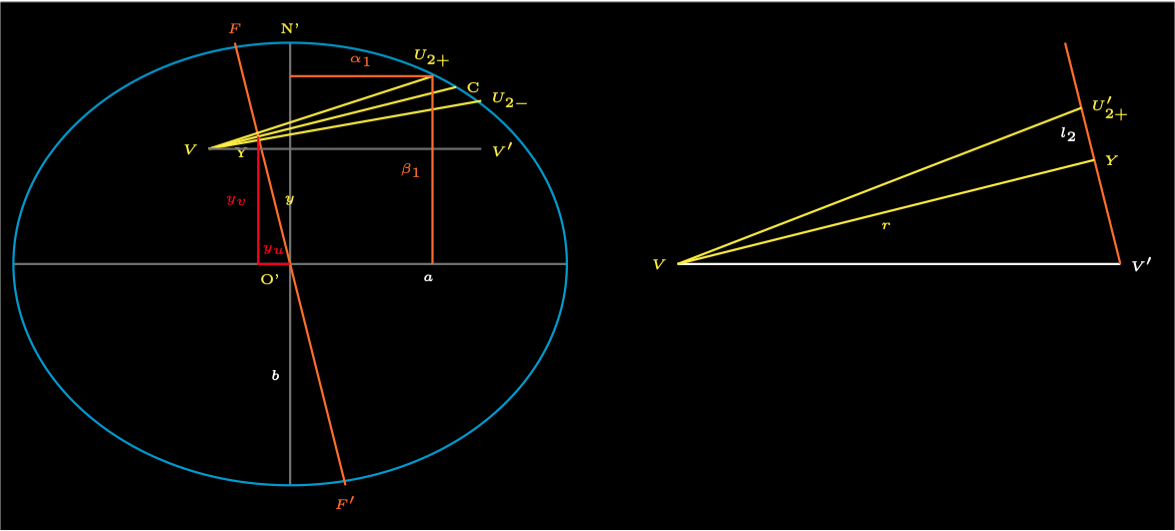
Figure 5: The Umbral Cone Width shows the intersection plane where the line \(VY\) is the shadow axis projected to the apex of the shadow cone. The points \(U_{2+}\) and \(U_{2-}\) are the points where the outer edges of the shadow cone intersect the Earth’s surface. The coordinates of point \(Y = (y_u, y_v) = (-y\sin d, y\sec d)\).

The angles \(\widehat{U_{2+}VC}\) and \(\widehat{CVU_{2-}}\) are both the besselian element \(f_2\).

The right of the diagram shows an expanding view of the diagram around the line \(VY\). The angle \(\widehat{YVV'}\) is the besselian element \(d\). The angle \(\widehat{U'_{2+}VY}\) is the besselian element \(f_2\). The distance \(YU'_{2+}\) is the besselian element \(l_2\). This is by convention negative for a total or annular eclipse, use the absolute value \(|l_2|\).

The distance \(VY = r = |l_2|\cot f_2\). Hence the coordinates of V can be calculated from point Y.

\[V = (v_u, v_v) = (\rho, \sigma) = (y_u -r\cos d, y_v - r\sin d) = (-y\sin d -|l_2|\cot f_2\cos d, y\sec d -|l_2|\cot f_2\sin d)\]

The gradient of the line \(VU_{2+}\) is \(\gamma = tan(d + f_2)\).

Use the tangent relationship.

\[\tan(d + f_2) = \frac{\tan d + \tan f_2}{1 - \tan d\tan f_2}\]

Use Equation (5) to Equation (11) to obtain the values of the latitude \(\phi\) longitude \(\lambda\).