
Mathematics
Tensor Calculus
Tensors were developed by Bernhard Riemann, Erwin Bruno Christoffel, Tulio Levi-Civita, and Gregorio Ricci-Curbastro to describe the differential geometry of multi-dimensional spaces.
Covariant and Contravariant Vectors
Consider a Cartesian frame of reference which has a ruler in it. We know that if one end of the ruler is at (0, 0) and the other end is at (a, b) then the length of the ruler s is:
\(s^2 = a^2 + b^2\)
Now consider an oblique frame of reference where the angle between the coordinate axes is latextmath:[\alpha].
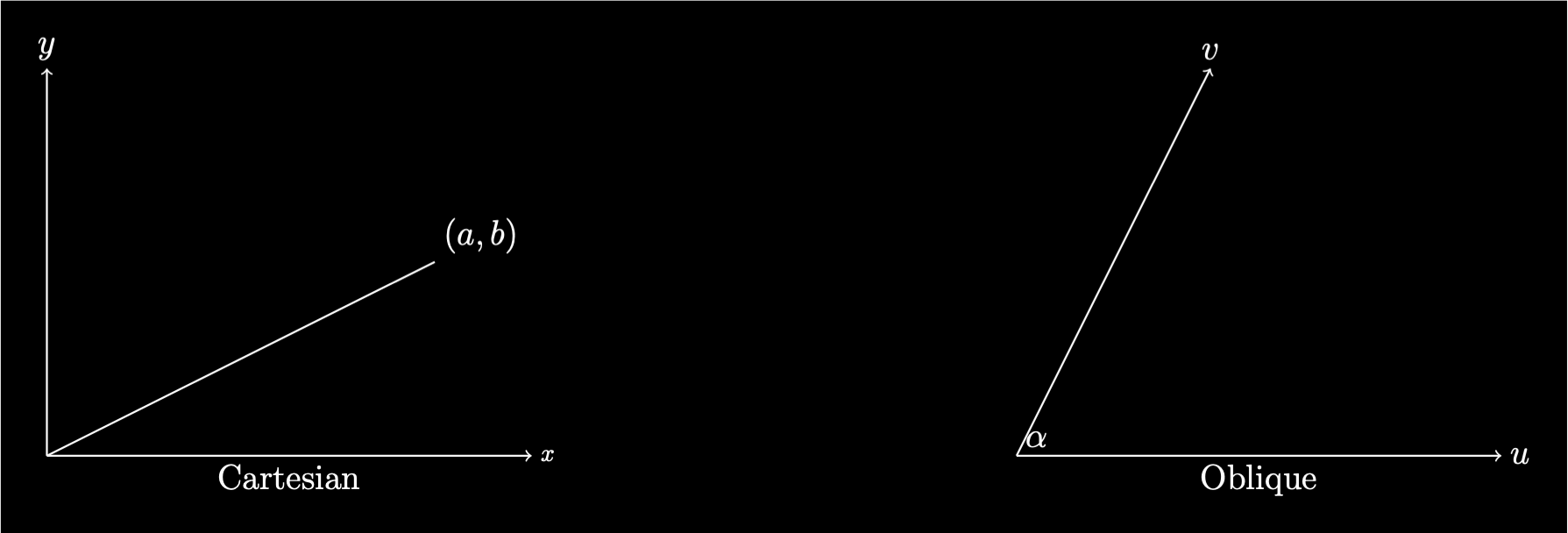
To get from one coordinate system to the other a transformation matrix has to be applied which transform the coordinate axes.
We now want to place the ruler in the oblique frame. There are two ways in which the end points can be transformed.
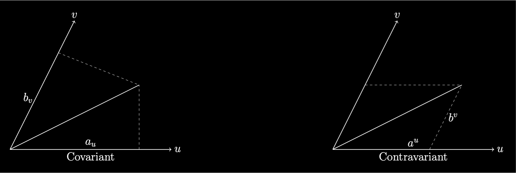
A covariant vector is obtained by applying the same transformation which was applied to the coordinate axes to a vector. The convention is that a covariant transformation is defined by using subscripts for the axes.
A contravariant vector is obtained by applying the inverse transformation to the transformation which was applied to the coordinate axes to a vector. The convention is that a contravariant transformation is defined by using superscripts for the axes.
The Cartesian length calculation gives a different result for both covariant and contravariant transformations. The length is preserved if by defining it in terms of both covariant and contravariant transformations.
\(s^2 = a^u a_u + b^v b_v = a^2 + b^2\)
Tensors
A tensor is effectively a multidimensional array. The rank of a tensor is the number of indexes required to uniquely identify an element. Tensors can contain scalars, vectors or other tensors. The notation for a tensor is a Latin or Greek letter with a number of indexes. The order of indexes is important. Each index is either a covariant subscript or a contravariant superscript. By convention Latin letters are used for indexes 1..3 and Greek letters for indexes 1..4. In equations containing tensors, if an index appears once in a term it is assumed to take all possible values. If an index appears exactly twice in a term it is assumed to be summed over all possible values. This is known as the Einstein Summation Convention.
Metric Tensor
A metric tensor is a function which enables the calculation of the distance between two points in a given space of any number of dimensions. It is often given the notation gij. The metric tensor is also used for the calculation of a distance given differential offsets in each dimension dxi.
\(ds^2 = g_{\alpha\beta}dx^\alpha dx^\beta\)
In Euclidean space the metric tensor is the Kronecker delta \(g_{ij} = \delta_{ij}\) which is 0 for \(i \neq j\) and 1 for i = j. In this case the distance is the familiar Pythagoras form.
\(ds^2 = \sum{dx_i^2}\)
The metric tensor is symmetric gij = gji. The inverse of the metric tensor is gij. The metric tensor can also be used to raise and lower indexes.
\(x_\alpha = g_{\alpha\beta}x^\beta\)
\(x^\alpha = g^{\alpha\beta}x_\beta\)
Christoffel Symbols
In order to do calculations on spaces it is necessary to define the derivatives with respect to the coordinates. This process was made easier by the German mathematician and physicist Elwin Bruno Christoffel. He introduced the Christoffel symbols which are defined in terms of the metric gij. They are used to study the geometry of the metric.
The Christoffel symbols of the first kind are tensor like objects \(\Gamma_{abc}\).
Christoffel symbols of the first kind can be defined in terms of the Christoffel symbols of the second kind \(\Gamma^m_{ij}\). The metric is used the raise or lower an index.
\(\Gamma_{ijk}=g_{mk}\Gamma^m_{ij}\)
Riemann Curvature Tensor
The Riemann curvature tensor describes the curvature of a manifold. It defines a tensor for each point on the manifold. It can be defined in terms of Christoffel symbols.
In four dimensions the Riemann tensor has 256 terms. It is however asymmetric in the first and second and the third and fourth indexes which reduces the unique components to 36.
\(R_{abcd} = -R_{bacd} = -R_{abdc}\)
It is also symmetric in the first and third and the second and fourth indexes which reduces the number of unique components to 21.
\(R_{abcd} = R_{cdab}\)
There is also an identity which reduced the number of unique indexes to 20.
\(R_{abcd} + R_{acdb} + R_{adbc} = 0\)
Levi-Civita Connection
This is where the works of Bernhard Riemann, Elwin Bruno Christoffel, Gregorio Ricci-Curbasto and Tulio Levi-Civita become entwined.
A parallel transport is the movement of a tangent vector along a closed curve on a manifold, keeping the tangent vectors parallel at all times. If the space is curved, when the tangent vector completes the transport it is pointing in a different direction to which it started. The angle difference is proportional to the area swept out. In fact the ratio of the angle to the area is the Ricci scalar R. The scalar is also the trace of the Ricci tensor Rij which will be described next. Notice the use of the metric to raise an index.
A connection is a more precise definition of a transport involving differentials. A metric connection is defined in terms of the inner product of any two vectors undergoing parallel transport is always the same. The Levi-Civita connection is a special case in that it is the unique torsion free metric connection. The torsion free condition means that the Christoffel symbols are symmetric.
\(\Gamma^i_{jk} = \Gamma^i_{kj}\)
The Levi-Civita connection is equivalent to the definition of the Christoffel symbols in terms of the metric.
Ricci Tensor
For any point on the surface of a manifold follow geodesics in all directions a short equal distance. The union of all of the end points is a geodesic ball. It can also be thought of as a ball made of a large number of flat surfaces.
The Ricci tensor \(R_{\mu\nu}\) represent the volume of a small wedge of a geodesic ball differs from that of a ball in Euclidean space.
The Ricci tensor can be defined in different ways. It can be a contraction of the Riemann tensor by summing over the first and third indexes.
\(R_{bd} = g^{ac}R_{abcd} = R^c_{bcd}\)
It can also be a contraction of the Riemann tensor by summing over the first and fourth indexes.
\(R_{bc} = g^{ad}R_{abcd} =R^d_{bcd}\)
It is important to identify the sign convention used to construct the Ricci tensor as \(g^{ac}R_{abcd} = -g^{ad}R_{abcd}\).
The Ricci tensor can be written in terms of the Christoffel symbols.
Ricci Scalar
The scalar curvature R is the difference in volume between a small geodesic ball in Riemannian space and the corresponding ball in Euclidean space. It is also referred to as the Ricci scalar.
\(R=g^{ij}R_{ij}=R^i_i\)
Stress Energy Tensor
The stress-energy tensor \(T_{\alpha\beta}\) describes energy, momentum, and flux, which is a flow of something. Electromagnetic fields behave like mass in some respects and curve space time.
Energy is usually regarded as a scalar quantity and momentum is a vector quantity. If the momentum vector is extended to four dimensions then energy can be placed in the time dimension. It acts as a form of pressure in the time direction. This four vector forms the first row and column of the stress-energy tensor.
The remaining components are the flows in different directions.
Static and Spherically Symmetric Body
A static and sperically symmetric body has a density \(\rho\) and a pressure p which are both functions of only the radius r. There is also assumed to be a relationship \(\rho = \rho(p)\).
The general form of the metric in polar coordinates is:
Where A = A(r) and B = B(r).
The stress-energy, or energy-momentum, tensor is:
\(T_{\mu\nu} = c^2((\rho + p)u_\mu u_\nu - pg_{\mu\nu})\)
Where \(u_\mu = (u_t, 0, 0, 0)\) and \(u^2_t = g_{tt}\).
Then the stress enery tensor is:
Electromagnetic Tensor
The electromagnetic tensor \(F^{\mu\nu}\) allows Maxwell’s equations to be simplified from four differential equations to two tensor equations. The electric field \(\mathbf{E}\) and the magnetic field \(\mathbf{B}\) can be written in terms of \(F^{\mu\nu}\).
\(E_i=cF_{0i}\) \(B_i= -\frac{1}{2}\epsilon_{ijk}F^{jk}\)
In spherical polar coordinates.
The stress-energy tensor is:
Maxwell’s Equations in Tensor Form
Pairs of Maxwell’s equations in differential form can be written as a single tensor equation. Take the first and fourth equations in terms of \(\mathbf{E}\) and \(\mathbf{B}\).
Where the four current \(J^\alpha\) is:
Take the second and third equations in terms of \(\mathbf{E}\) and \(\mathbf{B}\).
These can be written as the Bianchi Identity.